DATA SCIENCE USING PYTHON
ONLINE TRAINING COURSE
DECISION TREE MODELING USING PYTHON
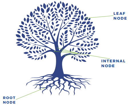
Some Keywords are related to the Decision Tree
To predict cases, decision trees use rules that involve the value of the input variables. The rules are arranged hierarchically in a tree-like structure with nodes connected by lines. The nodes represent decision rules and the lines order the rules.
The first rule at the top of the tree is called the root node. Subsequent rules are named internal or interior nodes. Nodes with only connection called leaf nodes. To score a new case, examine the input values, and apply the rules defined by the decision tree model.
Decision Tree model can be implemented in the following three steps:
1. Predict New Case: Before we build the model, we must clear about what our model is going to predict. There can be three types of predictions as follow:
- Decision — Your model uses inputs to make the best decisions for each case (For Example: classifying cases as a potential and non-potential customers)
- Ranking — Your model uses inputs to optimally rank each case. (For Example Model attempts to rank high-value cases higher than low-value cases.)
- Estimate — Your model uses inputs to optimally predicts the target value. (For Example, the average value of target for all cases having observed value of inputs in case your variable is numeric or probability of an event if your variable is categorical)
2. Input Selection: This step requires searching for inputs that are best in predicting (decision/ranking/estimate) the value of the response variable. This can be done by doing
- Input reduction — Redundancy in your dimension space and
-
Input reduction — Irrelevancy in your dimension space
3. Optimize complexity: Fitting a model requires searching through the space of possible models.
It involves a trade-off between bias and variance. An insufficiently complex model might not flexible enough, which can lead to underfitting that is systematically missing the signal (high bias).
People consider that the most complex model should always perform better than others. But the complex model might be too flexible which can lead to overfitting that is accommodating the nuances of error in a particular sample (high variance).
We must select the right amount of complexity which gives the best generalization.
- Predict New Cases
- Input Selection
- Optimize complexity
1. Predict New Cases
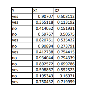
Let’s consider the binary response variable which has the value of “yes” or “no”. So, our model output will be a decision (either “yes” or “no”).
2. Input Selection
Decision Tree Modeling handles the curse of dimensionality problem by using three techniques.
Chi-square automatic interaction detection (CHAID):
As we are dealing with the interval scaled inputs, all the values of input variables serve as potential split points.
Let me put it by using two inputs x1 and x2 as follow:
For a selected data point for a specific input (say x1), two groups are generated. Cases with input values less than that data point are said to be branch left. Cases with input values greater than that data point are said to be branch right.
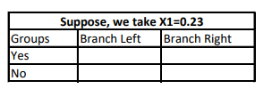
Now, we will simply fill the above 2*2 contingency table by calculating the proportion of the target outcome.
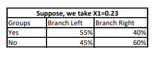
Once, we have this table, we will calculate the Pearson Chi-Square statistics is used to quantify the independence of counts in the table’s columns. A large value chi-square indicates that the proportion of yes in the left branch is different from the proportion of yes in the right branch. A large difference in the outcome proportion indicates a good split.
We will follow the same process to all other data points. As we will do multiple comparisons based on all other data points, the chances of type 1 error increases. Due to this, we will manipulate p-value using logworth = -log(chi-squared p-value).
Because each split point corresponds to a statistical test, the p-value needs to adjust by a factor equal to the number of tests being conducted. This inflated p-value is called as Bonferroni Correction.
For a split to occur, at least one logworth must exceed a threshold (one of the parameters in the decision tree model).
See it’s very simple provided you know the Pearson Chi-Square statistics in detail.
Entropy and Information Gain:
Entropy is the sum of the probability of each label times the log probability of that same label.
In the above 2*2 table for an X1 = 0.23, entropy is calculated as P(event) = proportion of event* log(proportion of event)
Now, for a split to occur, we will calculate as follow:
Entropy before the split occurs: As you can see we had 6 yes and 6 no in our original data. P(Yes) = 0.50 * log(0.50) and P(No) = 0.50 * log(0.50) and entropy_before = P(Yes)+P(No)
Entropy for Branch Left (that is X1 < 0.23): P(Yes) = 0.55 * log(0.55) then P(No) = 0.45* log(0.45) and entropy_left = P(Yes)+P(No)
Entropy for Branch Right(that is X1 > 0.23): P(Yes) = 0.40* log(0.40) then P(No) = 0.60* log(0.60) and entropy_right = P(Yes)+P(No)
Entropy After split:
We will now combine entropy_left and entropy_right that is entropy_after = entropy_left + entropy_right.
Now by comparing entropy_before and entropy_after we will get Information Gain that is information_gain = entropy_before — entropy_after.
Information gain measures how much information we gained by doing the split using that particular feature (X1 = 0.23). At each node of the tree, this calculation is performed for every feature, and the feature with the largest information gain is chosen for the split.
Gini:
Gini Index, also known as Gini impurity, calculates the amount of probability of a specific feature that is classified incorrectly when selected randomly. If all the elements are linked with a single class then it can be called pure.
Let’s perceive the criterion of the Gini Index, like the properties of entropy, the Gini index varies between values 0 and 1, where 0 expresses the purity of classification, i.e. All the elements belong to a specified class or only one class exists there. And 1 indicates the random distribution of elements across various classes. The value of 0.5 of the Gini Index shows an equal distribution of elements over some classes.
The Gini Index is determined by deducting the sum of squared of probabilities of each class from one, mathematically, Gini Index can be expressed as:
Gini Index = 1 — sum(P)**2.
While designing the decision tree, the features possessing the least value of the Gini Index would get preferred.
3. Optimize Complexity:
Decision tree modeling is a collection of different rules based on input space. We will find the right amount of complexity by assessing those rules on test or validation data. Different statistics can be used to measure the performance of the decision tree model. Again it is based on the prediction type and level of measurement of the target variable.
Here, we have a binary target variable with a prediction type equal to the decision. Appropriate statistics can be a number of true positives and a number of true negatives.
True Positives: matching primary decisions (yes) using your model with actual primary outcomes yields true positives.
True Negatives: matching secondary decisions (no) using your model with actual secondary outcomes yields true negatives.
Accuracy = tp + tn. We will analyze the accuracy using different numbers of rules (decision tree models) to set the right amount of complexity.
Let’s now implement it in Python. I tried to automate the entire process of the decision tree model as follow:
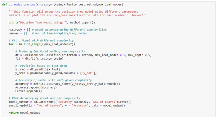
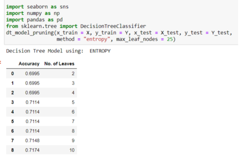
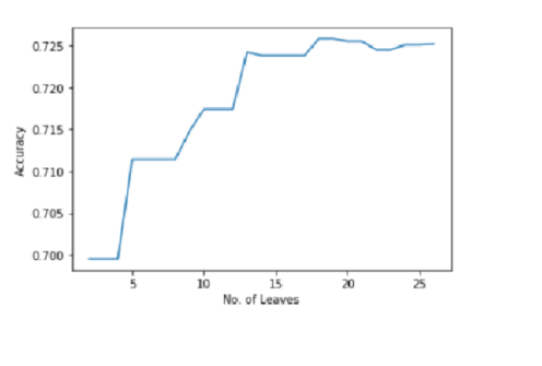
As it is clearly seen that Accuracy is a maximum nearby 18 leaf nodes tree. So, we will go with an 18 leaf decision tree. Some of the parameters from the script need clarity.
method = Criteria used to build a decision tree model. It is basically for Input/Feature Selection during the decision tree model development. Python sklearn only supports only entropy and gini. You can use gini too using this snippet.
max_leaf_nodes = Reduce the number of leaf nodes. This impacts the size of the tree.
max_depth = Reduce the depth of the tree to build a generalized tree. Set the depth of the tree to 3, 5, 10 depending after verification on test data