OLS (Ordinary Least Square) regression. OLS method finds the parameter estimates which reduces/optimizes the sum of squared error. The parameter estimates obtained using OLS are BLUE (Best Linear Unbiased Estimates). Let me expand the meaning of BLUE to understand the heart of this Post.

Best — Parameter Estimates obtained by using OLS has minimum variance compared to all other iterations/methods.

Linear — Parameter Estimates obtained using OLS are linear in parameters (all the parameters/betas are power raised to one.)

Unbiased — refers to the unbiased estimates.

The above properties are valid only if the below assumptions are met.

• Normality of residuals,
• Constant variance across the range of predicted values and
• Independence of residuals (means no error term provides any information about any other error term).

Now, let’s understand what will be the effect of violation of these assumptions.

1. Normality of residuals: It does not affect the parameter estimates meaning that OLS parameter estimates are still BLUE even if normality is violated. But it will affect the test results like t-test, F-test, chi-square test, and confidence interval of parameter estimates which requires normality assumption.
2. Homoscedascticity of variance: Again, it does not affect the parameter estimates but it affects the standard errors of the parameter estimates, and hence, it affects the test results as Std. Error is being used in CL, t-test, F-test, and so on. The model will suffer from Type 1 or Type 2 errors based on underestimate or overestimate of standard errors. The parameter estimates obtained are no longer BEST.
3. Independence residuals: Parameter estimates are not affected but Std. errors are compromised. Again Type 1 or Type 2 errors.

Most of the time, this is not straightforward and requires a different kind of transformations (Box-Cox, Log, Sqrt, Inverse, cross-product, and so on). We can also use WLS (Weighted Least Square Models) and Generalized Linear Models (Poisson, Negative Binomial, Gamma regression) and so on which doesn’t require the above assumptions.

If we try the above alternatives of transformation, we must back transform the model at the original scale with some adjustment factors which really increases the complexity. Even, GLM models require knowledge of specific statistics and their complexities. WLS also requires the proper estimation of weights.

Now, see below the sample output:

The second and third assumptions affect the Standard Error of the parameter estimates which is highlighted above. It means that if we correct/adjust the standard error of parameter estimates, then we never require transformations or any other modeling techniques.

How to correct/adjust the Standard Errors of parameter estimates?

Standard Error of OLS estimators are calculated using

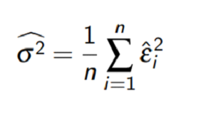
We can estimate sigma square using

And hence, Standard error of OLS estimators are

White (1980) adjusted the covariance matrix as below so that Standard error will be no longer compromised.

Let’s implement it using some data. I used the polynomial regression model to model the price of the car based on highway mileage and horsepower (maximum horsepower)

HC Std. Error is different from usual Std. Error from OLS. In the presence of heteroskedasticity, use the HC standard error and test results based on that. You can also select the variables/features based on this HC standard error and test results based on that.

Correcting the heteroskedasticity using this method does not require any back transformation or any adjustment factor. This method is widely used in time series analysis and econometrics.

Hope it provides a good alternative to transformations or different models if OLS assumptions are not met.